An introduction to Filters

While filters have always been a part of the Profiler, they are now partly exposed only with the upcoming 0.8.7 version. Shortly explained: filters are algorithms of different nature which can be applied to portions of data. The starting point to interact with filters is the filter view. This view is triggered with the Ctrl+T shortcut. Let’s start with some step by step screenshots.

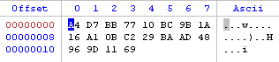
This is a Zip file and the gray area marks a compressed file. Let’s select this area with Ctrl+Alt+A.

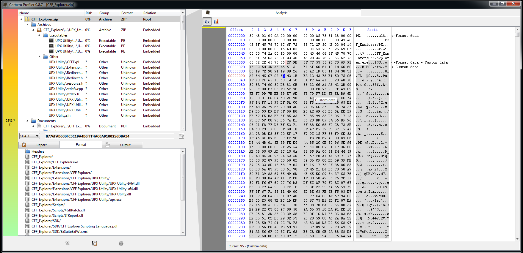
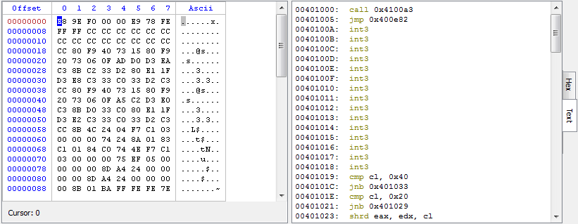
Now let’s press Ctrl+T and take a look at the filter view.

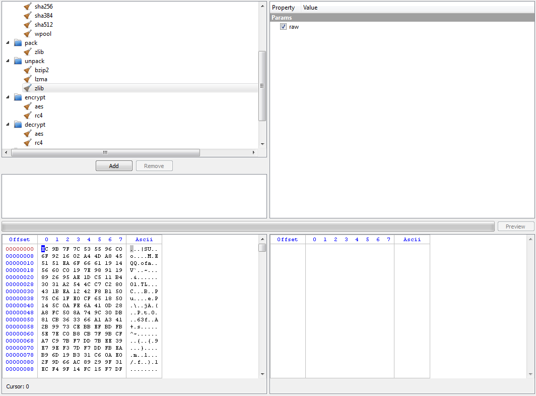
The tree at the top-left displays the available filters. The property editor next to it contains the available parameters for the currently selected filter and the list beneath the filters is the stack of filters which need to be applied to the input data. The hex view on the left contains the data which we have previously selected in the hex view (meaning the compressed file) and represents the input data.

Now if we want to decompress the data, let’s add the unpack/zlib filter (with the raw parameter checked) to the stack by clicking on “Add”.

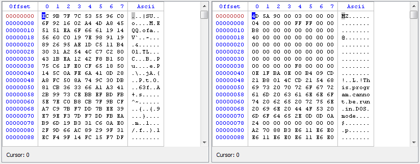
And at this point we can click on the “Preview” button.

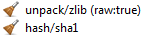
But what if we want to retrieve the SHA1 of the decompressed data? Just add the hash/sha1 filter to the stack.

This time we’ll have only the SHA1 hash in the output view.

The filter stack can be imported and exported. Just right-click inside the stack list. The exported filters of the current stack will look like this:

If we had opened the filter view without a selection we would have had an editable hex view on the left, which we could fill with our custom data. Also, the hex views in the filter view have all the benefits of a regular hex view (that is if the filter view is not triggered while loading a file, as we’ll see later); this means that it’s possible to trigger a new filter view by selecting something in the hex view containing the filtered output data.

What I’ve showed until now isn’t an every-day task, but it serves the purpose of introducing the topic. We’ll see some real-word cases after I have introduced the misc/basic filter. But before of that let me shortly mention text output filters.

Right now the Profiler features two filters with text output: disasm/x86 and disasm/x64. When a filter outputs text, we’ll be shown by default a text view instead of the hex view on the right.

This can come handy when decrypting shellcode. What we also most probably need is the misc/basic filter, which I think will be one of the most commonly used filters. Let’s look at its parameters.

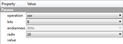
operation specifies what is going to be performed on the input data. Available operations are: set(fill), add, sub, mul, div, mod, and, or, xor, shl, shr, rol, ror. bits specifies the size in bits of each element the operation has to be performed on (values up to 64 bit are supported). endianness applies only to elements greater than 8 bits. radix is related to the input format of value. value contains the data used for the operation.

If I now inserted “FF” as value, then I would be xoring every byte of the input data with that 1-byte value. If, however, I inserted “FF 00”, then I would be xoring every even byte with “FF” and every uneven one with “00”. I may even only modify every third byte by using wildcards and leaving the first two unchanged, I only have to insert “* * FF”. Wildcards and arrays can be used even in the context of values bigger than 1 byte of course.

Now that I’ve introduced the basic filter, let’s see our first real-world case. What you see is a PDF containing an encrypted malware.

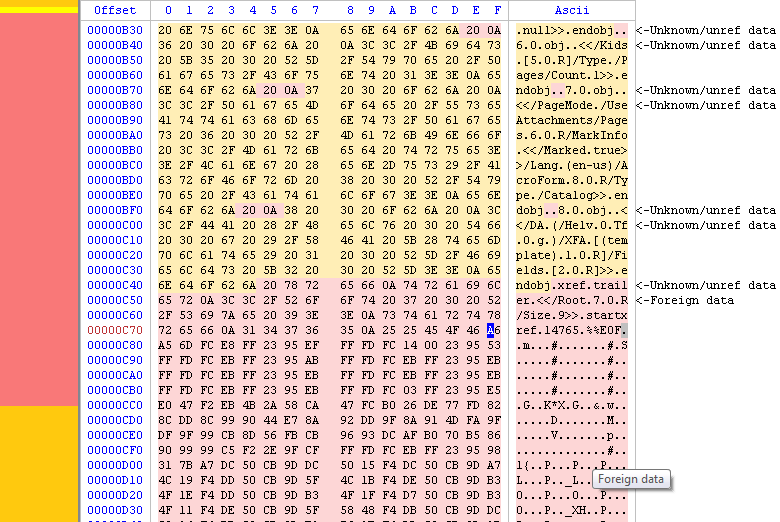
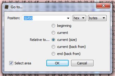
At the caret position an encrypted Portable Executable starts, it’s quite easy to figure out because of the repetitive sequence of bytes (a PE header is full of zeroes). I select the data with the go to dialog (Ctrl+G).

Now instead of triggering the filter view directly, I’m going to load the embedded file with Ctrl+E. This triggers the load file dialog.

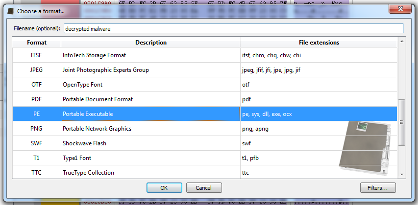
As you can see I specified the format of the file to load (PE) and inserted an optional name for it, but now it’s necessary to tell the Profiler how to decrypt the file, otherwise it won’t be able to load it. So I’ll just click on the “Filters” button at the bottom-right and a filter view dialog will pop up.

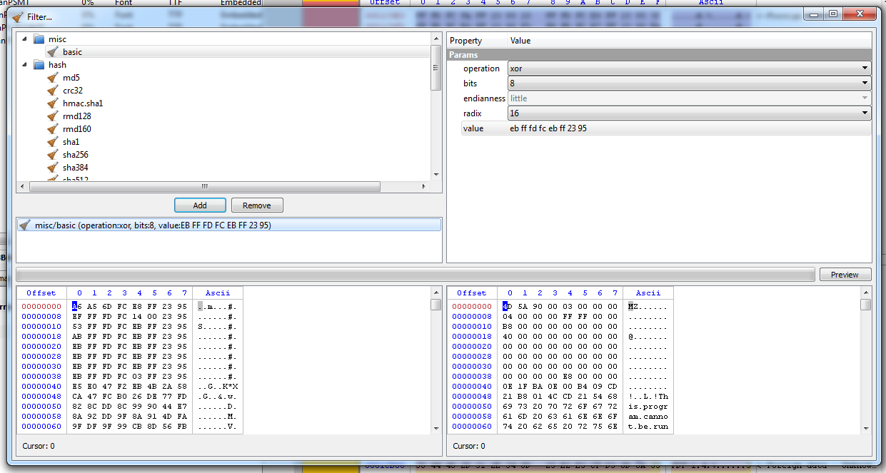
The decryption sequence is “EB FF FD FC EB FF 23 95”. It can be expressed like I did as an array.

But since it amounts to a 64-bit value, it can also be expressed like this.

Ok, back to the malware. After having added the decryption filter to the stack I just close the dialog and confirm the load file dialog. We’re now able to navigate the decrypted PE.

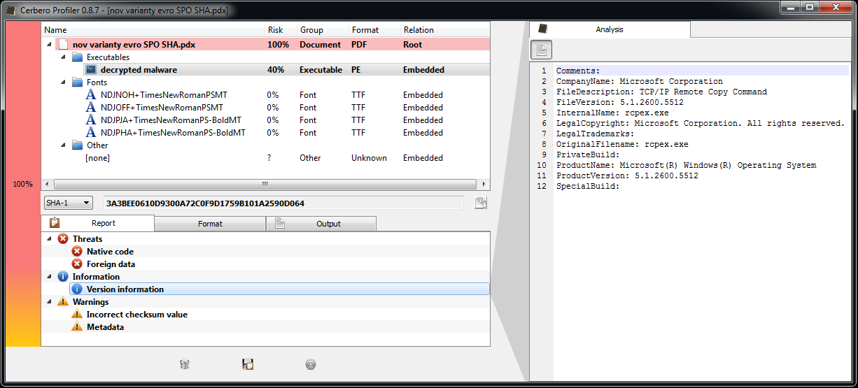
Now I can just save the project (which is under 1KB) and send it to a colleague who will be able to inspect the decrypted file.

The last real-world case I’m going to present I made it myself, because it was easier than to start looking for one. I just took a cursor resource from a PE and appended another RC4-encrypted PE to it. Then replaced the original resource and opened the host file with the Profiler.

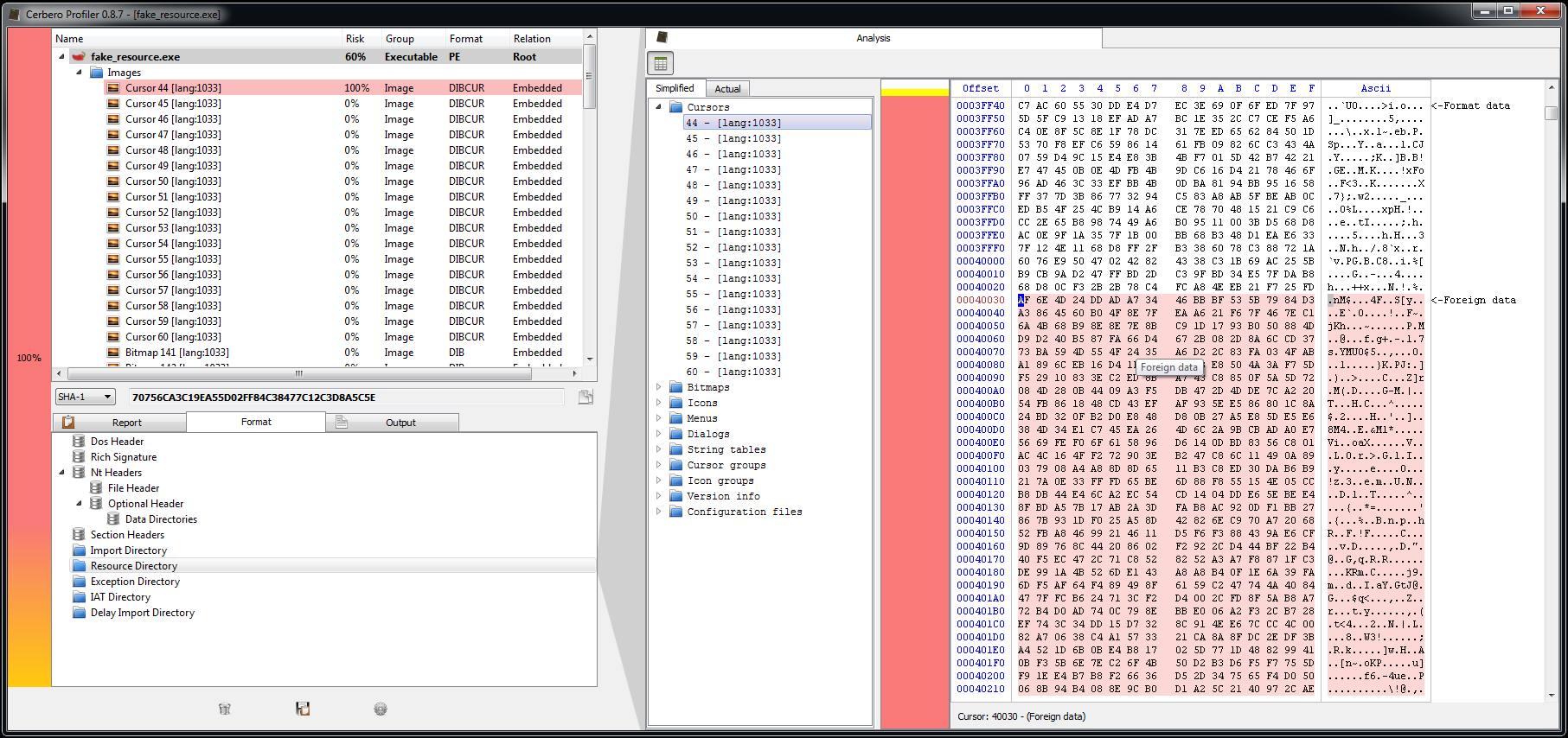
The Profiler tells us that the are problems in the resource and also shows us the file. In fact, we can see where the foreign data begins. I just select the foreign data (I can do this both from the resource directory or from the DIBCUR embedded file), trigger the load file dialog and apply the decryption filter.

In upcoming updates there will be many improvements to filters: many more will be added and the concept will be extended and made customizable. Clearly this post doesn’t cover all of that, but I think for now this is enough to keep the introduction simple.