This is the first of a series of posts which will be dedicated to PE analysis features. In previous posts we have seen how the Profiler has started supporting PE as a format and while it still lacks support for a few directories (and .NET), it supports enough of them for x86 PE analysis.
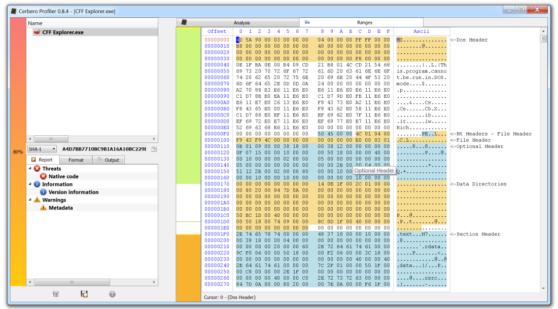
While the upcoming version 0.8.4 of the Profiler also features analysis checks as CRC, recursion, metadata, etc., this post will be about the in-depth range analysis for PE files. As the screenshot above previews, in-depth ranges show PE data structures in a hex view and the distribution of data in a PE file.
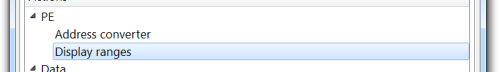
Let’s take as first sample “kernel32.dll”. After having it opened in the Profiler, let’s execute the “PE->Display ranges” action.
We get the PE ranges for kernel32.
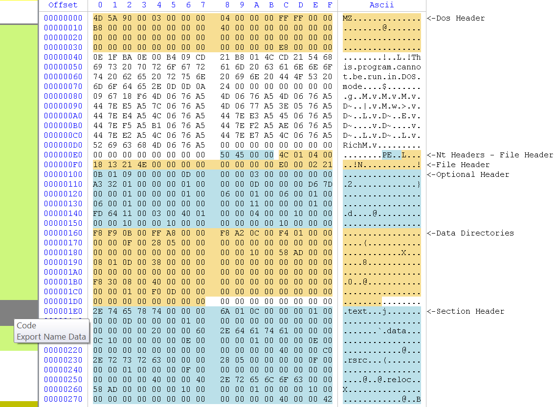
The big region of data marked as fluorescent green represents executable code. As you can see, it is interrupted by a gray region of data which the tooltip tells us being a combination of “Code” and “Export Name Data”. If we move the cursor, we can see that it’s not only Export data, but also Import data. Which means that the Export and Import directory are contained in the executable part of the file (the IAT is in the thin gray area at the beginning of the code section). But we may not be interested in having the code section covering other data regions. This is why we can filter what we want to see (Ctrl+B).
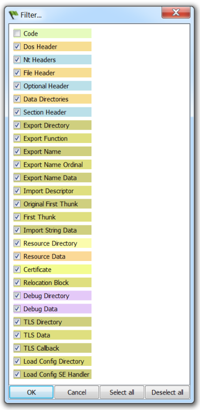
I unmarked the “Code” range. Thus, we now get all the ranges except the unmarked one.

We can also jump to regions of data, but before seeing that, I want to briefly mention that the hex view can be printed to file/PDF or captured.
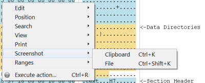
Not a big feature, but it may come handy when generating reports.
Now let’s look at a file I have especially crafted for the occasion, although it reflects a very common real-world case.

We’ve got a PE with an extremely high quantity (50%) of foreign data and the entropy level of that data is also extremely high.
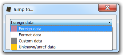
So let’s jump to the first occurrence of foreign data (Ctrl+J).
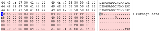
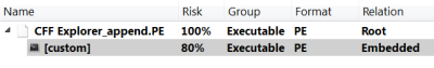
What we see is that right there where the analyzed PE files finishes, another one has been appended.
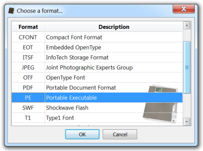
So let’s select the contiguous range of data (Ctrl+Alt+A: this will select the foreign range of data) and “Load selection as…” (Ctrl+E) will asks us to select the file type to load (it is automatically identified as being a PE).
We are now able to analyze the embedded PE file.
While this procedure doesn’t highlight anything new, since loading of embedded files has been featured by the Profiler from its earliest versions, I wanted to show a practical use of it in connection with ranges.
It has to be noted that this particular case is so simple that it can be detected automatically without interaction of the user. In fact, detection of appended files in PEs will be added most probably in version 0.8.5.
Hope you enjoyed this post and stay tuned for the next parts!
PS: take advantage of our promotional offer in time. Prices will be updated in August!
Great job! Congratulations Daniel!